X-Ray Diffraction Residual Stress Techniques

GENERAL USES

Determination of residual stresses from lattice strain in crystalline materials:

Macrostress measurement

• Nondestructive surface residual stress measurement for quality control.
• Determination of subsurface residual stress distributions
• Measurement of residual stresses associated with failures caused by fatigue or stress corrosion

Microstress measurement

• Determination of the percent cold work at and below the surface
• Measurement of hardness in steels in thin layers

EXAMPLES OF APPLICATIONS

• Determination of the depth and magnitude of the compressive layer and hardness produced by carburizing steels
• Investigation of the uniformity of the surface compressive residual stresses produced by shot peening in complex geometries
• Measurement of surface residual stresses and hardness on the raceway of ball and roller bearings as functions of the hours of service
• Study of the alteration of residual stress and percent cold work distributions caused by stressrelieving heat treatment or forming
• Measurement of surface and subsurface residual stresses parallel and perpendicular to a weld fusion line as a function of distance from the weld
• Determination of the direction of maximum residual stress and percent cold work gradient caused by machining

SAMPLES

• Form: Polycrystalline solids, metallic or ceramic, moderate to fine grained
• Size: Various, with limitations dictated by the type of apparatus, the stress field to be examined, and x-ray optics
• Preparation: Generally, none. Large samples and inaccessible areas may require sectioning with prior strain gaging to record the resulting stress relaxation. Careful handling or protective coatings may be required to preserve surface stresses

LIMITATIONS

• Expensive, delicate apparatus generally limited to a laboratory or shop
• Only shallow (<0.025 mm, or 0.001 in.) surface layer is measured, requiring electrolytic polishing to remove layers for subsurface measurement
• Samples must be polycrystalline, of reasonably fine grain size, and not severely textured

ESTIMATED ANALYSIS TIME

1 min. to 1 hr. per measurement, depending on the diffracted x-ray intensity and technique used. Typically, 1 hr. per measurement for subsurface work, including material removal and sample repositioning

CAPABILITIES OF RELATED TECHNIQUES

Linear Elastic Diffraction Techniques calculating stress from total elastic strain:

• Neutron Diffraction: Residual stress is calculated from the strain measured in the crystal lattice by neutron diffraction. Essentially the same Bragg’s Law diffraction process as x-ray diffraction, but using the de Broglie wavelength of thermal neutrons from a reactor. Neutron penetration is on the order of centimeters for common metals, allowing three dimensional stresses to be determined, but the unstressed lattice spacing must be known independently.

Linear Elastic Mechanical Techniques calculating stress from relaxed elastic strain:

• General Dissection Techniques: Determination of residual stress distributions from strain relaxation or deflection caused by sectioning or removing layers from the sample. Some symmetry and uniformity of the residual stress field is generally assumed. Classic methods (Stabline’s, Letner’s, Sach’s methods) are restricted to simple geometries, such as beans, plates, cylinders or tubes for which closed form stress solutions of stress from the measured strain are available. Finite element solutions are now in use for more complex geometries and stress fields.
• Center Hole Drilling: Applicable to a variety of samples and materials with stress fields uniform over dimensions larger than the strain-gage rosette dimensions and depth of the drilled hole. Stress magnitude must be less than nominally 80% of yield strength to avoid errors due to local yielding at the hole. Non-uniformity of the stress field near a free edge, eccentricity of the hole, and residual stresses induced in drilling the holes are sources of error. Principal stress distributions can be determined with depth up to several mm by incremental drilling, with accuracy limited at the surface where relaxation is minimal. Widely used and supported commercially. See ASTM E837-13a.
• Ring Core: The incremental ring-core method, also referred to as the trepan method, is a widely used mechanical residual stress measurement method. The technique consists of machining an annular groove around a strain gage via electrical discharge machining (EDM) or milling. The change in strain is monitored as a function of cut depth. The method provides a comprehensive assessment of the resolved and principal residual stress field as a function of depth. The ring-core technique can be used on metals, ceramics, and polymers, where linear elastic theory can be assumed.
• Deep Hole Drilling: Provides principal stress distributions in high depth resolution along the length of a hole drilled deep into the sample. Strain relaxation is measured with an air gauge as the change in diameter in multiple orientations at each depth increment after trepanning or coring around the hole to relax the residual stresses. Principal stresses are calculated from the diametral strains in three orientations at each depth. DHD is applicable to a wide variety of machinable material. Depth is limited only be the length of the tooling. Data cannot be obtained within approximately 1 mm of the surface.
• Contour Method: The sample is through sectioned on a plane by wire EDM exposing a cut face. The contours on the cut face caused by relaxation of residual stress acting normal to the face are measured by laser or mechanical means. The residual stress distribution normal to the cut face is approximated by a finite element model of the strains required to restore the contoured plane. Results depend upon data smoothing and the functional form of the stress model assumed. Accuracy near the free surface is limited due to distortion at the start of EDM cuts.
• Slitting Method: A functional form for an equilibrium residual stress distribution in one dimension on a plane through the sample is approximated by series solutions from strain relaxations measured by strain gages placed near slits cut on either the front or back face of the sample. Mathematically stable solutions are limited by the order and type of series assumed and prior data smoothing. Limited to one dimensional stress fields and full equilibrium solutions. Non-Linear Elastic Methods calculating stress from other stress dependent properties:
• Ultrasonic Methods: Stress is estimated from changes in the speed of sound propagated through the material by pressure waves or along the surface by shear waves. Sensitivity varies greatly with material. Relatively long gage lengths and stress-free reference standards are required. Of limited general application due to errors caused by transducer coupling, preferred orientation, cold work, temperature, and grain size. Speed and nondestructive nature are a benefit in process monitoring applications.
• Magnetic (Barkhausen or Magnetostrictive) Methods: Limited to ferromagnetic materials and subject to many of the limitations and error sources of ultrasonic methods. Highly nonlinear response with low sensitivity to compressive stresses. Limited in general laboratory applications because of variation in transducer response and magnetic coupling. Depth sampled depends upon frequency. Nondestructive and fast for process monitoring of both residual stress and hardening of steels.

 

INTRODUCTION

Residual stresses are generally caused by non-uniform thermal and/or mechanical plastic deformation as in forming, machining, grinding, shot peening, welding, quenching, or virtually any thermal-mechanical process that leaves a distribution of elastic strains. Phase transformations that produce non-uniform volume changes in a part, as in carburizing or case hardening of steel or austenite transformations in service, also generate residual stresses, generally compressive, in the expanding hardened layer. Although non-uniform plastic strain or phase changes produce residual stresses, once the part is in equilibrium, the residual stresses produced are entirely elastic. The prior complex thermal-mechanical history and plastic strain details of casting, forging, forming, heat treatment or machining need not be known. Only the elastic strains remaining in the free part at thermal equilibrium contribute to the residual stress distribution in the part.

Although the term residual stress “measurement” is widely used, stress is an extrinsic property that is not directly measurable. All methods of stress determination require measurement of some intrinsic properties, such as strain and elastic constants, or force and area, from which the associated stress is calculated. X-ray and neutron diffraction methods calculate the residual stress from the elastic strain measured in the crystal lattice without altering the part. Mechanical methods calculate the residual stress from the change in strain relaxed (or dimensional change) caused by sectioning, slitting, drilling or trepanning the part. The nonlinear elastic methods including Barkhausen noise, eddy current and ultrasonic rely upon higher order effects of stress upon the magnetic, electrical or acoustical properties of the part.

If the part is not externally constrained, then the residual stress distribution must be in equilibrium. Equilibrium requires that the integral of the forces and the moments acting on any entire plane through the body must both sum to zero. It is not necessary that the residual stress at any one point that happens to be measured must show equilibrium with depth into the part. For example, if a point in the center of a plate is heated to incandescence and cools, then it will be the residual tension entirely thought the thickness, surrounded by equilibrating residual compression. A bend formed in a tube will be in tension through the wall that was deformed in compression, and in residual compression through the side deformed in tension. Cross-roll straightened bar stock will have spiral patterns of residual tension and compression. The complex residual stress distribution in a weld depends upon the geometry, constraints, order of fusion, temperature distribution and cooling. There is really no limit to the complexity of residual stress distributions that can be formed, but they must always be in elastic equilibrium.

Mechanical methods of residual stress measurement are limited by assumptions concerning the nature of the residual stress field and sample geometry. Being necessarily destructive, mechanical methods cannot be directly checked by repeat measurement. The residual stress is calculated from the strain or deflection produced by sectioning to relax the residual stresses present. Only in the limit of relaxing all of the residual stress in the body can the true residual stress present be determined. The sample geometry is usually limited to simple forms (plates, beams, cylinders, etc.) by the availability of closed form solutions to calculate residual stress from the measured change in strain. Finite element solutions can be developed for more complex geometries. Spatial and depth resolution are generally an order of magnitude less than those of x-ray diffraction.

All nonlinear elastic methods are subject to major error from material properties. Variation in preferred orientation, cold work, hardness, and grain size can affect the properties measured orders of magnitude more than residual stresses present. All require stress-free reference samples, which are otherwise identical to the sample under investigation. Nonlinear elastic methods find application for nondestructive process monitoring, such as monitoring induction hardening, where the sample geometry and material properties are consistent. They are generally not suitable for general laboratory residual stress determination. In addition, their spatial and depth resolutions are much less than x-ray diffraction.

X-ray diffraction residual stress methods calculate the residual stress present from the strains measured in the crystal lattice of the grains in the sample. Because the residual stresses are entirely elastic, the entire stress present is measured nondestructively without altering the sample. To determine the stress in one direction on the sample surface, the strain in the crystal lattice must be measured for at least two precisely known orientations relative to the sample surface. Therefore, x-ray diffraction residual stress measurement is applicable to materials that are crystalline, relatively fine grained, and produce diffraction for any orientation of the sample surface. Samples may be metallic or ceramic, provided a diffraction peak of suitable intensity and free of interference from neighboring peaks can be produced in the high back-reflection region with the radiations available. X-ray diffraction residual stress measurement is unique in that macroscopic and microscopic residual stresses can be determined nondestructively, but only in a very thin layer, nominally 0.01mm (0.0005 in.) deep.

Macroscopic stresses, or macrostresses, which extend over distances that are large relative to the grain size of the material, are of general interest to engineers. These are the stresses of primary interest in component design, finite element analysis, and fatigue or stress corrosion failures. Macrostresses are homogeneous, in the sense that they extend uniformly over the various metallurgical features of grains, grain boundaries, and precipitates. Macrostresses are second order tensor quantities, with shear and normal stress magnitudes both varying in three directions at a single point in a body. The macrostress for a given location and direction is determined by measuring the strain in that direction at a single point. When macrostresses are determined in at least three known directions, and a condition of plane stress is assumed at the free surface, the three stresses can be combined using Mohr’s circle for stress to determine the maximum and minimum residual stresses, the maximum shear stress, and their orientation relative to a reference direction. Macrostresses strain many crystals uniformly in the surface. This uniform elongation or compression of the crystal lattice shifts the angular position of the diffraction peak selected for residual stress measurement. The lattice strain is calculated from the small angular shift in the position of the diffraction peak. The residual stress in the surface is calculated from the strain measured in crystals oriented at two or more angles to the surface.

Microscopic stresses, or microstresses are inhomogeneous, varying over minute distances in both magnitude and orientation. Microstresses exist between different phase particles, regions of different crystallographic orientation, and the sub-grain regions between dislocation tangles. The literature contains various attempts to classify microstresses as different types, and to relate them to the phase selective xray diffraction measurement of lattice strain and residual stresses. Inter-phase stresses result from different states of stress in the phases present in the sample matrix. Examples are stresses developed between the martensite and austenite phases after heat treatment of steel, or between precipitates and the matrix phase of an alloy. Because XRD stress measurement is inherently phase selective, any measurement is for the one diffracting phase. This make XRD methods unique in being able to measure the different phase stresses separately. But it must be kept in mind when interpreting the results obtained on multiphase materials that the stress of only one phase may be known. Other than the inter-phase stresses, microstresses cannot be measured directly in the minute individually stressed regions.

Diffraction Peak Breadth is of more practical use as a measure of the effect of microstresses on the broadening of the diffraction peak. The aggregate effect on the range of lattice strain can then be treated as a scalar property of the material in the diffracting volume. The percent of cold work or hardness are scalar properties without direction that result from dislocations and imperfections in the crystal lattice causing the microstresses. Diffraction line broadening is associated with strains in the regions between dislocation tangles within the crystal lattice that traverse distances much less than the dimensions of the crystals. Broadening of the diffraction peaks used for macroscopic residual stress measurement arises from variation in the local lattice spacing of the “coherent diffracting domains” or crystallites, the perfectly crystalline material between dislocations, and from the range of strains in these regions. Compressively stressed crystallites contribute to the high angle side of the peak, and tensile regions to the low angle side. Measurable broadening of the diffraction peak from the related reduction in crystallite size begins as the domains become smaller than a few hundred atomic dimensions, insufficient to ensure the constructive and destructive interference of Bragg’s Law. A scalar measure of the range of microstresses can be determined from the diffraction-peak breadth measured in conjunction with macroscopic residual stress measurement. The peak breadth can be related empirically to material properties useful in materials engineering, including cold work level, yield strength and hardness.

Principles of X-Ray Diffraction Stress Measurement

In x-ray diffraction residual stress measurement, the strain in the crystals making up the sample itself provides the “strain gage” needed to calculate the residual stresses present. The method uses linear elastic theory to calculate stress from strain, but on an atomic scale, rather than the mm scale of electrical resistance strain gages. Therefore, samples must be crystalline, fairly fine grained, and not too highly oriented so that well defined diffraction peaks are produced by many crystals at any angle to the surface. Fortunately, most high strength forgings and machined or shot peened surfaces meet these requirements. Coarse grained materials, such as castings, may not be suitable.

The selective nature of x-ray diffraction allows the spacing of a specific set of crystal lattice planes (h k l) oriented at a precise angle to the sample surface to be measured with the accuracy needed to determine the strain in the surface. Figure 1 shows the diffraction of a monochromatic beam of x-rays at a high diffraction angle, 2θ, from the surface of a stressed sample for two orientations of the sample relative to the x-ray beam. The angle ψ, defining the orientation of the sample surface, is the angle between the normal of the surface and the incident and diffracted beam bisector, which is also the angle between the normal to the diffracting lattice planes and the sample surface.

 

Figure 1: Principles of X-ray Diffraction Residual Stress Measurement D, x-ray detector; S, x-ray source; N, normal to the surface (a) Ψ = 0: Poisson’s ratio contraction of lattice spacing (b) Ψ > 0: Tensile extension of lattice planes by stress σ

 

Diffraction occurs at an angle 2θ, defined by Bragg’s Law: nλ = 2d sin θ, where n is an integer denoting the order of diffraction, λ is the x-ray wavelength, d is the lattice spacing of crystal planes, and θ is the diffraction angle. For the monochromatic x-rays produced by the metallic target of an x-ray tube, the wavelength is known to 1 part in 10⁵ . Any change in the lattice spacing, d, results in a corresponding shift in the diffraction angle 2θ. The angular shift in the position of a typical diffraction peak with a half-width of several degrees is generally less than a degree, requiring high accuracy in sample placement, peak location and angular measurement.

Figure l (a) shows the sample in the ψ = 0 orientation. The presence of a tensile stress in the sample results in a Poisson’s ratio contraction, reducing the lattice spacing and slightly increasing the diffraction angle, 2θ. If the sample is then rotated through some known angle ψ (Fig. 1b), the tensile stress present in the surface increases the lattice spacing over the stress-free state and decreases 2θ. Measuring the change in the angular position of the diffraction peak for at least two orientations of the sample defined by the angle ψ enables calculation of the stress present in the sample surface lying in the plane of diffraction, which contains the incident and diffracted xray beams. To measure the stress in different directions at the same point, the sample is rotated about its surface normal to coincide the direction of interest with the diffraction plane.

Because only the elastic strain changes the mean lattice spacing, only elastic strains are measured using x-ray diffraction for the determination of macrostresses. When the elastic limit is exceeded, further strain results in dislocation motion, disruption of the crystal lattice, and the formation of microstresses, but no additional increase in macroscopic stress. Although residual stresses result from nonuniform plastic deformation, all residual macrostresses remaining after deformation are necessarily elastic.

The residual stress determined using x-ray diffraction is the arithmetic average stress in a volume of material defined by the irradiated area, which may vary from square centimeters to square millimeters, and the depth of penetration of the x-ray beam. The linear absorption coefficient of the material for the radiation used governs the depth of penetration, which can vary considerably. However, in iron, nickel, and aluminum-base alloys, 50% of the radiation is diffracted from a layer approximately 0.005 mm (0.0002 in.) deep for the radiations generally used for stress measurement. This shallow depth of penetration allows determination of macro and microscopic residual stresses as functions of depth, with depth resolution approximately 10 to 100 times that possible using other methods.

Although in principle virtually any interplanar spacing may be used to measure strain in the crystal lattice, availability of the wavelengths produced by commercial x-ray tubes limits the choice to a few possible planes. The choice of a diffraction peak selected for residual stress measurement impacts significantly on the precision of the method. The higher the diffraction angle, the greater the precision. Practical techniques generally require diffraction angles, 2θ, greater than 120°.

Table I lists recommended diffraction techniques for various alloys. The relative sensitivity is shown by the value of K45, the magnitude of the stress necessary to cause an apparent shift in diffraction-peak position of 1° for a 45°ψ tilt. As K45 increases, sensitivity decreases.

Plane-Stress Elastic Model

The radiations suitable for x-ray diffraction (XRD) stress measurement are very “soft”, with low energies (typically 5 to 8 KeV) and wavelengths comparable to the lattice spacing to be measured. The diffraction peaks then occur at high Bragg angles, providing maximum lattice strain resolution. The soft x-ray penetration is very shallow and attenuated exponentially. Nearly all of the diffracted radiation comes from a layer only about 0.025 mm (0.001 inch) thick in most materials of engineering interest, confining the measurement to the very near surface of the sample. Electropolishing is used to remove successive layers exposing new surfaces for subsurface measurement. Corrections for the exponential attenuation of the radiation penetrating the subsurface stress distribution and for relaxation of the stresses present due to layer removal are then necessary, as discussed below. The shallow x-ray penetration gives much higher depth resolution than other methods. Because the surface is not disturbed in order for the lattice strain to be measured, XRD stress measurement is the only method that can measure the actual surface stress nondestructively.

 

Fig. 2 -Plane-stress elastic model

 

The diffracting surface layer is so thin that a condition of plane stress can be assumed to exist at this free surface. That is, a stress distribution described by principal stresses σ1, and σ2 exists in the plane of the surface, and no stress, normal or shear, is acting perpendicular to the unrestrained free surface, σ3 = 0. A strain component 3 does exist normal to the surface as a result of the Poisson’s ratio contractions caused by the two principal stresses shown in Figure 2.

 

ε_φψ = [(1 + ν)/E (σ₁α₁² + σ₂α₂²)] − [ν/E (σ₁ + σ₂)]

Equation 1

where E is the modulus of elasticity, ν is the Poisson’s ratio, and α1 and α2 are the angle cosines of the strain vector:

 

α₁ = cos φ sin ψ
α₂ = sin φ sin ψ

Equation 2

Substituting for the angle cosines in Equation 1 and simplifying enables expressing the strain in terms of the orientation angles:

 

ε_φψ = [(1 + ν)/E (σ₁ cos²φ + σ₂ sin²φ) sin²ψ] − [ν/E (σ₁ + σ₂)]

Equation 3

If the angle ψ is taken to be 90°, the strain vector lies in the plane of the surface, and the surface stress component, σφ is:

 

σ_φ = (σ₁ cos²φ) + (σ₂ sin²φ)

Equation 4

Substituting Equation 4 into Equation 3 yields the strain in the sample surface at an angle φ from the principal stress σ1:

 

ε_φψ = [(1 + ν)/E σ_φ sin²ψ] − [ν/E (σ₁ + σ₂)]

Equation 5

Equation 5 relates the surface stress σφ, in any direction defined by the angle ψ, to the strain , in the direction (φ,ψ) and the principal stresses in the surface. Note that Equation 5 describes any elastic plane stress condition at a surface regardless of how the stresses might be measured.

XRD stress measurement is now introduced through the use of the strain measured in the crystal lattice. If dφψ is the spacing between the lattice planes measured in the direction defined by φ and ψ, the strain can be expressed in terms of changes in the linear dimensions of the crystal lattice:

ε_φψ = Δd/d₀ = (d_φψ − d₀)/d₀

where d0 is the stress-free lattice spacing. Substitution into Equation 5 yields:

 

(d_φψ − d₀)/d₀ = [(1 + ν)/E]_(hkl) σ_φ sin²ψ − [ν/E]_(hkl) (σ₁ + σ₂)

Equation 6

where the elastic constants \((1 + \nu/E)_{(hkl)}\) and \((\nu/E)_{(hkl)}\) are not the bulk values but the values for the crystallographic direction normal to the lattice planes in which the strain is measured as specified by the Miller indices (hkl). Because of elastic anisotropy, the elastic constants in the (hkl) direction commonly vary significantly from the bulk mechanical values, which are an average over all possible directions in the crystal lattice.

The lattice spacing for any orientation, then, is:

d_φψ = [(1 + ν)/E]_(hkl) σ_φd₀sin²ψ − [(ν/E)_(hkl)d₀(σ₁ + σ₂) + d₀]

Equation 7

Equation 7 describes the fundamental relationship between lattice spacing and the biaxial stresses in the surface of the sample. The lattice spacing \(d_{\phi\psi}\), is a linear function of \(\sin^2\psi\). Figure 3 shows the actual dependence of d(311) for \(\psi\), ranging from 0 to 45° for shot peened 5056-O aluminum having a surface stress of -148 MPa (-21.5 ksi), to which a straight line has been fitted by least squares regression.

 

Fig. 3 – A d(311) versus \(\sin^2 \psi\) plot for a shot peened 5056-O aluminum alloy having a surface stress of -148 MPa (-21.5 ksi)

 

The intercept of the plot at \(\sin^2 \psi = 0\) is:

which equals the unstressed lattice spacing, \(d_0\), minus the Poisson’s ratio contraction caused by the sum of the principal stresses. The slope of the plot is:

σ_φ = (E/(1 + ν))_(hkl) (1/d₀) (∂d_φψ/∂sin²ψ)

Equation 9

The x-ray elastic constants can be determined empirically, but the unstressed lattice spacing, d0, is generally unknown, and may depend upon local composition. However, because E » (σ1 + σ2), the value of dφ0 from Equation 8 differs from d0 by not more than ± 1%, and σφ, may be approximated to this accuracy using:

 

σ_φ = (E/(1 + ν))_(hkl) (1/d_φ0) (∂d_φψ/∂sin²ψ)

Equation 10

The XRD method then becomes a differential technique, and no stress-free reference standards are required to determine d0 for the biaxial stress case. The three most common methods of x-ray diffraction residual stress measurement, the single-angle, two-angle, and sin2 ψ techniques, assume plane stress at the sample surface, and are based on the fundamental relationship between lattice spacing and stress given in Equation 7. The residual stresses of interest in the sample surface and with depth by electropolishing, can be determined accurately even if the nominal lattice spacing varies with alloying, carburizing, or cold work. The XRD method is a differential technique requiring only the measurement of lattice spacing at two or more angles to the surface.

In contrast, neutron diffraction or XRD techniques using high energy synchrotron radiation that penetrates deep into the surface cannot assume that plane stress exists in the diffracting volume. To calculate the residual stresses from the lattice strains, the full stress tensor must be solved and the unstressed lattice spacing must be independently known, which may be impractical in inhomogeneous materials, like a case hardened steel.

If the lattice spacing is determined not be a linear function of sin2 ψ then the XRD method should not be attempted. Nonlinear d vs sin2 ψ dependence can be due to shear stresses acting out of the surface, or extreme preferred orientation, but this is very rarely seen in practice. Nonlinearity is most commonly caused by: 1) instrument misalignment, 2) poor x-ray optics, 3) grain sizes too coarse to produce well defined peaks, 4) poor diffraction peak locating algorithms, 5) severe preferred orientation causing variation in the elastic constants with ψ , 6) non-uniform stress in the irradiated area varying with ψ . In such cases, simply fitting a straight line by linear regression to the data will not produce a valid result.

The single-angle technique, or single-exposure technique, derives its name from early photographic methods that require a single exposure of the film. (Ref 1,2) Position sensitive detectors have replace x-ray film. The method is generally considered less sensitive than the two-angle or sin2 ψ techniques primarily because the possible range of ψ is limited by the diffraction angle 2θ, but it has the advantage of not requiring any instrumental movements. Figure 4 shows the basic geometry of the method.

 

Fig. 4 – Basic geometry of the single-angle technique for x-ray diffraction residual stress measurement Np, normal to the lattice planes; Ns, normal to the surface. See text for a discussion of other symbols. Source: Ref 2

 

Figure 4 shows the basic geometry of the method. A collimated beam of x-rays is inclined at a known angle, \(\beta\), from the sample surface normal. X-rays diffract from the sample, forming a cone of diffracted radiation originating at point 0. The diffracted x-rays are recorded using film or position-sensitive detectors placed on either side of the incident beam. The presence of a stress in the sample surface varies the lattice spacing slightly between the diffracting crystals shown at points 1 and 2 in Fig. 4, resulting in slightly different diffraction angles on either side of the x-ray beam. If \(S_1\), and \(S_2\) are the arc lengths along the surface of the film or detectors at a radius R from the sample surface, the stress is:

 

σ_φ = (E/(1 + ν))_(hkl) × (S₁ − S₂)/(2R) × cot θ/(sin²ψ₁ − sin²ψ₂)

Equation 11

The angles ψ1, and ψ2 are related to the Bragg diffraction angles θ1, θ2, and the angle of inclination of the instrument, β, by:

 

ψ₁ = β + θ₁ − π/2

And

ψ₂ = β + θ₂ − π/2

The precision of the method is limited by the principle that increasing the diffraction angle \(2\theta\) to achieve precision in the determination of lattice spacing reduces the possible range of \(\sin^2\!\psi\), lessening sensitivity. The single-angle technique is generally not used, except for film and position-sensitive detector apparatuses designed for high-speed measurement.

Cosine Alpha Technique.

The Cosine Alpha method is instrumentally similar to the Single-Angle technique, and was first developed in Japan initially to measure the stress in extremely small irradiated areas for the purpose of mapping stresses around the tip of cracks in fatigue crack growth samples. (Ref 3) The technique uses data from the entire Debye ring collected with a two-dimensional area detector positioned where the cone of diffraction intersects the plane of the two detectors (or film strips) shown in Figure 4. The peak positions at four quadrants of the Debye ring are measured, and the stress is calculated in two directions on the surface. Although commercial instruments are offered, the literature describing the means of calculating the stresses and the potential experimental errors are limited. Sensitivity of the stresses reported to the precise position of the incident beam position and the angle ψ are noted, but no quantitative assessments or comparison to other techniques are currently available. The Cosine Alpha method does not appear to offer a significant advantage over the conventional XRD methods described below, if a sufficient diffracted beam intensity is available.

Two-Angle Technique

Equation 7 and Figure 3 show that if the lattice spacing, dφψ, is a linear function of sin2 ψ, the stress can be determined by measuring the lattice spacing for any two ψ angles. In this respect, the Two-Angle technique is similar to the Single-Angle, but ψ values can be selected to provide optimal sensitivity or to avoid interference with the x-ray beam. The technique has been thoroughly investigated by the Society of Automotive Engineers (SAE) and is widely accepted.(Ref 4) Selecting ψ angles to provide as large a range of sin2 ψ as possible within the limitations imposed by the diffraction angle 2θ and the sample geometry maximizes sensitivity of the method. Lattice spacing is determined precisely at two extreme values of ψ, typically 0 and 45°, and the stress is calculated using Equation 10. Because only the slope of d vs sin2 ψ is required to calculate the stress, it is easily shown that the accuracy of measurements using just the two extreme ends of the sin2 ψ range is comparable to least squares fitting to numerous points, provided dφψ, is a linear function of sin2 ψ.

The sin2 ψ technique

(Ref 4) is identical to the two-angle technique, except lattice spacing is determined for multiple ψ tilts, a straight line is fitted by least squares regression (as shown for the shot peened aluminum sample in Figure 3), and the stress is calculated from the slope of the best fit line using Equation 10. The method is a standard procedure that is widely used and described in SAE H784 and European specification BS EN 15305:2008. It requires measurement time in proportion to the number of ψ tilts used. Positive ψ tilts are recommended due to the increased experimental error associated with negative values. The method provides no significant improvement in accuracy over the two-angle technique using the two ψ tilts at the extreme ends of a linear d vs sin2 ψ range. It but does allow nonlinearity to be detected, and is recommended when initially investigating measurement of samples that may have large grain size. The primary benefit of the sin2 ψ technique, considering the additional time required for data collection, is in establishing the linearity of d as a function of sin2 ψ to demonstrate that x-ray diffraction residual stress measurement is possible on the sample of interest. As noted, XRD measurements should not be attempted if the dependence is not linear. Simply fitting a line to nonlinear data, which unfortunately is commonly observed, will not produce a valid stress value.

The Marion-Cohen technique

characterizes the dependence of lattice spacing on stress in highly textured materials. (Ref 5) The method assumes a biaxial stress field with an additional dependence of the lattice spacing on a texture distribution function f (ψ), a measure of the (hkl) pole density calculated from the diffracted intensity over the range of ψ tilts used for stress measurement. The model assumes a lattice spacing dependence of:

 

d_φ0 = ((1 + ν)/E)_(hkl) σ_θd₀sin²ψ + (d_max − d_β)f(ψ) + d_β

Equation 12

where dmax and dB are the maximum and minimum lattice spacings in the range investigated. The method requires simultaneous determination of the preferred orientation, or texture, in the sample to determine f (ψ) along with lattice spacing, and is solved by multiple linear regression over the functions f (ψ) and dψφ as functions of sin2 ψ to determine σφ, dmax, and dB.

The assumption that the lattice spacing and preferred orientation present at the time of measurement resulted entirely from the same origin limits practical application of the method. Residual stresses produced by shot peening, grinding, or machining in most materials of practical interest yield virtually identical results when measured by the MarionCohen, two-angle, and sin2 ψ methods. (Ref 6)

Full-Tensor Determination.

An expression for the lattice spacing can be formulated as a function of φ and ψ, assuming that a triaxial rather than plane stress state may exist in the layers penetrated by the x-rays below the free surface. Shear and normal stresses may then exist in all directions, as in neutron diffraction from the sample interior. Triaxial stresses in the surface layers penetrated by the x-ray beam is a possible explanation for nonlinear dependence of the lattice spacing on sin2 ψ reported in severely ground steel or shot peening at steep angles. Nonlinearities in the form of elliptical curvature of the d vs sin2 ψ plots resulting in “ψ splitting” are attributable to shear stresses σ13 and σ23, acting normal to the surface, where σ33 is the stress normal to the surface. All three must be zero at the free surface in plane stress. Psi splitting results in different values of the lattice spacing for positive and negative ψ tilts, and potential error in stress calculation if linearity is assumed.

In principle, the full-tensor method(Ref 7, 8) can determine the near surface stresses without assuming plane stress at the free surface. However, extensive data collection is required, generally exceeding that acceptable for routine testing. True “ψ splitting” caused by out-of-plane shear stresses will cause an elliptical separation of positive and negative ψ data. Subsurface stress gradients in plane stress will also cause nonlinear d vs sin2 ψ plots, but the curvature is the same for positive and negative ψ tilts. Before the full tensor methods can be applied, the raw data must first be corrected for penetration of the x-ray beam into the subsurface stress gradient. Unfortunately, sample and instrumental misalignment, x-ray beam divergence, stress gradients along the surface or with depth, and peak location errors can produce similar nonlinearity. Using only positive ψ tilts and comparing data for φ = 0 and 180 degree sample orientations eliminates the instrumental contributions, allowing true ψ splitting to be detected.

Unlike the plane-stress methods, determination of the full stress tensor requires absolute knowledge of the unstressed lattice spacing, d0, at the accuracy required for strain measurement (1 part in 105 ) to calculate the stress tensor from the measured strains. In many cases, such as for plastically deformed surfaces generated by machining or

⟨ε⟩_φψ =

⟨d_φψ⟩ − d₀


d₀

= A(τ)[(ε₁₁(z)cos²φ

+ ε₁₂(z) sin 2φ + ε₂₂(z)sin²φ)sin²ψ

+ (ε₁₃(z) cos φ

+ ε₂₃(z) sin φ)sin 2ψ + ε₃₃(z)cos²ψ]

 

composition gradients in carburized steels, the lattice spacing varies as a result of deformation or heat treating, precluding independent determination of the unstressed lattice spacing with sufficient precision. The extensive data collection and dependence on absolute knowledge of d0 limit the full-tensor method primarily to research applications.

X-Ray Integral Method

Studies have been directed at developing nondestructive residual stress measurement x-ray diffraction (NRSM-XRD) methods of recovering the underlying residual stress distribution from measured nonlinear lattice spacing vs. sin2 ψ data. Work prior to 1989 is reviewed by Eigenmann, Scholtes and Macherauch.(Ref 19) Attempts have been made to estimate both high stress gradients and shear components acting normal to the surface through the depth of penetration of the x-ray beam. All such methods assume some functional form to describe the subsurface strain (or stress) distribution, and seek to find the form of that function which best describes the observed attenuation weighted integral of lattice spacing with depth. The true strain or stress subsurface distribution (z-profile) is calculated from the measured weighted integral of the lattice spacing with depth (τ-profile).

A method capable of recovering a generalized approximation of the stress function has been described by Wern and Suominen.(Ref 20) The method, known as the X-Ray Integral Method, abbreviated as RIM, is a means of nondestructive determination of the full triaxial state of stress within the depth of the x-ray penetration, allowing for both a full stress tensor and variation in all of the stress components with depth. Published results show that the necessary equilibrium condition (σ33 = 0 at the surface) is achieved in the preliminary tests, even though this condition is not required by the method of solution. The method also does not depend upon lattice spacing measurements at extremely small grazing angles, minimizing defocusing errors in peak location, error due to surface roughness, and the difficulties of the LaPlace transform solution method.

The RIM method allows calculation of residual stresses from strain distributions measured as a function of depth below the surface. The method is based upon approximating the unknown z-profile of strain, ε(z), shown in Equation 13, using Fourier trigonometric series expansion. No prior knowledge of the residual stress distributions is required; the stress distribution is not forced to follow a linear pattern. Standard x-ray diffraction equipment can be used to collect the data.

The average measured strain profile can be expressed as a function of τ where D is the information depth defined by the penetration of the diffracted x-rays and z is the depth below the surface of the specimen.

 

⟨ε_φψ⟩(τ) = (∫₀^D e^−z/rε(z) dz)/(∫₀^D e^−z/r dz)

Equation 13

The equation of x-ray strain determination is shown as

where A(τ) is the integral operator in Equation 13 and Ψ and Φ are the angles that define the direction of strain measurement in the sample coordinate system. A system of m equations with n unknowns can be established by substituting a Fourier series description of the strain distribution with depth for each of the six strain profiles shown in Equation 14. Direct methods of solving for the unknown coefficients in the system of equations in general fail due to the nearly singular condition of the matrix. A technique known as the method of conjugate gradients can be used to determine the coefficients of a poorly conditioned set of equations.

 BASIC PROCEDURE

Sample preparation, if the geometry of the sample does not interfere with the incident or diffracted x-ray beams, is generally minimal. Preparation of the sample surface depends on the nature of the residual stresses to be determined. If the stresses of interest are produced by such surface treatments as machining, grinding, or shot peening, the residual stress distribution is usually limited to less than 500 µm of the sample surface. Therefore, the sample surface must be carefully protected from secondary abrasion, corrosion, or etching. Samples should be oiled to prevent corrosion and packed to protect the surface during handling. Secondary abrasive treatment, such as wire brushing or sand blasting, radically alters the surface residual stresses, generally producing a shallow, highly compressive layer over the original residual stress distribution.

If the stresses of interest are those produced by carburizing or heat treatment, it may be advisable to electropolish the surface of the sample, which may have undergone finish grinding or sand blasting after heat treatment. Electropolishing eliminates the shallow, highly stressed surface layer, exposing the subsurface stresses before measurement.

To measure the inside surface of tubing, in bolt holes, between gear teeth, and other restrictive geometries, the sample must be sectioned to provide clearance for the incident and diffracted x-ray beams. Unless prior experience with the sample under investigation indicates that no significant stress relaxation occurs upon sectioning, electrical resistance strain-gage rosettes should be applied to the measurement area to record the strain relaxation that occurs during sectioning. Unless the geometry of the sample clearly defines the minimum and maximum directions of stress relaxation, a full rectangular strain-gage rosette should be used to calculate the true stress relaxation in the direction of interest from the measured strain relaxation.

Following x-ray diffraction residual stress measurements, the total stress before sectioning can be calculated by subtracting algebraically the sectioning stress relaxation from the x-ray diffraction results. If only near-surface layers are examined on a massive sample, a constant relaxation correction can be applied to all depths examined. If a significant volume of material is removed, as in determination of the stress distribution through the carburized case of a thin bearing race, a more accurate representation of sectioning relaxation can be achieved by applying strain-gage rosettes to the inner and outer surfaces and by assuming a linear relaxation of stress through the sample.

Sample Positioning. Because the diffraction angles must be determined to accuracies of approximately ±0.01°, the sample must be positioned in the x-ray beam at the true center of rotation of the ψ and 2θ axes, and the angle ψ must be constant throughout the irradiated area. Therefore, extremely precise positioning of the sample to accuracies of approximately 0.025 mm (0.001 in.) is critical. Further, the size of the irradiated area must be limited to an essentially flat region on the sample surface. Small diameter samples or such sample geometries as small-radius fillets, the roots of threads, and fine-pitched gears may contribute to major sources of error if the x-ray beam is not confined to an essentially flat region at a known ψ tilt on the curved surface. If the irradiated area is allowed to span a curved surface, ψ will not be constant during determination of lattice spacing. These restrictions imposed by the sample geometry may prohibit x-ray diffraction residual stress measurement in many areas of primary concern, such as the roots of notches.

As the irradiated area is increased, the diffracted beam intensity increases, and the data collection time necessary to achieve adequate precision for residual stress measurement diminishes. The precision with which the diffracted intensity can be determined varies as the inverse of the square root of the number of x-rays collected. To determine the intensity to an accuracy of 1% at a single point on the diffraction peak, 104 x-rays must be counted, regardless of the time required. With diffracted intensities typically available on a fixed slit diffractometer system, this may require collection times of approximately 30 s for each point on the diffraction peak. If seven data points are collected on each diffraction peak for a two-angle technique, total measurement time may be 10 to 15 min. Reducing the irradiated area sufficiently to decrease the diffracted intensity by an order of magnitude increases the data collection time proportionally for the same precision in measurement. If high background from sample fluorescence in the x-ray beam is not a problem, positionsensitive detectors can be used to collect data simultaneously at numerous points across the diffraction peak, with some sacrifice in angular precision, reducing data collection time by an order of magnitude.

Diffraction-Peak Location.

To achieve the lattice strain resolution and accuracy required for XRD residual stress measurement, diffraction peaks with widths of several degrees must be located with a precision on the order of 0.01 degree. A variety of mathematical methods have been developed to locate diffraction peaks, with varying degrees of success. The calculated diffraction angle positon can shift as the shape of the diffraction peak changes as ψ is changed. As material is removed by electropolishing for subsurface measurement, the shape of the diffraction peak changes as the hardness in case hardened steels or cold working of machined or shot peened surfaces varies with depth. Reported nonlinear d vs sin2 ψ behavior is more often caused by instrument alignment or inaccurate diffraction peak location than stresses acting out of a free surface. Errors in locating the diffraction peak are a primary source of experimental error in XRD stress measurement.

The transition metal targets of the x-ray tubes used for stress measurement produce a continuous spectrum of white radiation and three monochromatic high-intensity lines. The three lines are the Kα1, Kα2, and Kβ characteristic radiations with wavelengths known to high precision. The Kα1, and Kα2 lines differ too little in wavelength and energy to allow separation of the diffraction peaks produced. The highest intensity Kα1 line is nominally twice the intensity of the Kα2 line, making it the preferred wavelength for residual stress measurement. The higher energy Kβ line has a significantly shorter wavelength, and can generally be separated from the Kα lines by filtration, the use of detectors with high-energy resolution, or crystal diffracted beam monochromators. The Kβ line intensity is typically one fifth that of the Kα1 line, and is generally too weak for practical x-ray diffraction residual stress measurement on plastically deformed surfaces.

Because the Kα doublet is generally used for residual stress measurement, the diffraction peaks produced consist of a superimposed pair of peaks, as shown in Figure 5 for four cases, indicating the various degrees of broadening that may be encountered. The variable blending of the Kα doublet typical of an annealed sample is indicated by curve A; a fully hardened or cold-worked sample, curve D. Because the accuracy of x-ray diffraction residual stress measurement depends on the precision with which the diffraction peak can be located, the method used to locate broadened doublet peaks is of primary importance.

 

Fig. 5 -Range of Kα doublet blending for a simulated steel (211) Cr Kα peak at 156.0°. A, fully annealed, B and C, intermediate hardness; D, fully hardened

 

Precise determination of the position of the diffraction peak at each ψ tilt begins with collection of raw intensity data at several points on the peak. The diffracted intensity (x-rays counted per unit time) or inverse intensity (time for a fixed number of x-rays to be counted) is determined to a precision exceeding 1% at several fixed diffraction angles, 2θ, spanning the diffraction peak. Depending on the method to be used for peak location, 3 to 15 individual data points and 2 background points are measured using standard diffractometer techniques. If data are collected using a position-sensitive detector, the diffracted intensity can be determined at dozens of data points spanning the diffraction peak. Sharp diffraction peaks, such as those shown in curve A in Fig. 5, may be located using intensity data of lower precision than that required for broad peaks, as shown in curve D. The number of x-rays to be collected, and therefore the time required for stress measurement to a fixed precision, increases as the diffraction peaks broaden.

Before determining a diffraction-peak position, the raw measured intensities must be corrected for Lorentz polarization and absorption. A sloping background intensity is then corrected by subtracting the background, assuming a linear variation beneath the diffraction peak. Various numerical methods are available to calculate the position of the diffraction peak. The simplest method, incorporated in early automated diffraction equipment, is to locate 2θ positions on either side of the peak at which the intensity is equal and assume the peak position to be at the midpoint. A straight line can be fitted to the opposing sides of the diffraction peak and the point of intersection of the two lines taken as a peak position (Ref 10). Early SAE literature recommends calculating the vertex of the parabola defined by three points confined to the top 15% of the peak (Ref 11). A significant improvement in precision can be achieved, approaching the 0.01° resolution of most diffractometers, by collecting 5 to 15 data points in the top 15% and fitting a parabola by least squares regression before calculation of the peak vertex.

If the intensity is measured at many points ranging across the entire Kα doublet, the peak position can be calculated as the centroid of the area above the background or by autocorrelation. Both of these area-integration methods are independent of the peak shape, but are extremely sensitive to the precision with which the tails of the diffraction peak can be determined. and therefore to the accuracy of the background correction.

All the above methods are effective, regression fit parabola being superior, if applied to a single symmetrical diffraction peak profile, such as the simple Kα1, peak shown in curve A in Fig. 5 or the fully combined doublet shown in curve D. All can lead to significant error in the event of partial separation of the doublet, as shown in curve B (Fig. 5). Partial separation commonly results from defocusing as the sample is tilted through a range of ψ angles. If residual stresses are measured as a function of depth, diffraction peaks can vary from breadths similar to curve D (Fig. 5) at the cold-worked surface through a continuous range of blending to complete separation beneath the cold-work layer, as shown in curve A. All the techniques of peak location discussed can lead to significant error in stress measurement as the degree of doublet separation varies.

The Rachinger correction (Ref 12) can be applied to separate the Kα doublet before fitting parabolas, but the precision of the correction diminishes on the Kα2 side of the combined profile and is generally inadequate for precise residual stress measurement. Fitting Pearson VII distribution functions (Cauchy to Gaussian bell-shaped, as described in Ref 13 and 14) separately to the Kα1 and Kα² diffraction peaks, assuming a doublet separation based on the difference in wavelength, provides a method of peak location that overcomes most of the problems outlined above.

 

Fig. 6 Comparison of d (21.3) versus sin² ψ data taken 0.176 mm (0.0069 in.) below the surface for a ground Ti-6Al-4V sample using two diffraction peak location methods

 

Figures 6 and 7 show the effect of the peak-location method on the results obtained. Figure 6 illustrates comparison of the same data reduced using Pearson VII distribution functions and a five-point least squares parabolic fit for ground Ti-6Al-4V using the (21.3) planes for residual stress measurement. Apparent nonlinearities in d versus sin2 ψ for the parabola fit are due to inaccurate diffraction-peak location in the presence of partial blending of the Kα doublet. Figure 7 shows the errors in stress measurement by the two methods of peak location applied to the identical data for the entire stress profile. The errors for the distribution function fit are smaller than the plotting symbols at all depths. Notice that even the sign of the residual stress calculated is effected by the peak location method.

 

Fig. 7 -Comparison of residual stress patterns derived using Cauchy and parabolic peak location for a ground Ti-6Al-4V sample using a six-angle sin² ψ technique. Errors in stress measurement by two methods of diffraction-peak location are shown.

 

Microstress Determination and line Broadening.

Diffraction peak broadening is caused by imperfections in the crystal. Plastic deformation creates and drives dislocations through the crystalline grains breaking them into smaller “crystallite” or “coherent diffracting domain” regions of perfect crystalline stacking order between the dislocation tangles. Phase transformations, notably the martensitic and austenitic phases in steels, produce comparable affects. As the dislocation density increases, these diffracting regions become smaller. When smaller than about 1000 atomic layers, the crystalline structure is no longer sufficiently periodic to support Bragg’s Law, and the peaks become broader. In addition to reduced crystallite size, the difference in lattice strain between the individual elastically deformed crystallites causes further broadening by contributing diffracted intensity to opposing sides of the diffraction peak. Tensile strained regions diffract to the low side, and compressive regions to the high angle side. The individual crystallite “microstresses” cannot be measured individually, but the range of microstress can be assessed in terms of the diffraction peak broadening.

The contributions to diffraction peak broadening can be separated into components due to strain in the crystal lattice and size. First, the broadening which is of instrumental origin must be separated from that due to crystallite lattice strain and size using Fourier analysis of the diffraction-peak profile and data collection sufficient to define the precise shape of the entire diffraction peak. Analysis of the Fourier series terms then allows separation of the components of broadening attributable to lattice strain from that caused by reduction in the crystallite size. However, this method requires extensive data collection, and is very dependent upon the precision with which the tails of the diffraction peak can be separated from the background intensity.

For most routine analyses of microstresses associated with cold working or heat treatment separation of the strain and size components is not necessary, and much simpler determinations of diffraction-peak breadth are adequate. The diffraction-peak breadth can be quantified either as the integral breadth (total area under the peak divided by diffraction-peak height) or the width at half the height of the diffraction peak. The width of the diffraction peak can be calculated directly from integrated data points or from the width of the function fitted to the diffraction-peak profile during macrostress measurement. Microstresses and macrostresses can then be determined simultaneously from the peak breadth and position.

Figures 8 and 9 show empirical relationships established between diffraction-peak breadth at half height for the (211) peak for M50 high-speed tool steel as a function of hardness and for the (420) peak breadth as a function of percent cold work for René 95, respectively. These empirical curves can be used to calculate the hardness or percent cold work in conjunction with macroscopic measurement. For the percent cold work curve, samples are heat treated, then deformed in tension, compression, or combined means to produce a series of coupons with various known amounts of cold work. Note that because cold work is defined in terms of the true plastic strain, the peak width is independent of the mode of deformation and is cumulative.(Ref. 14) Because the initial heat treatment may alter significantly the initial peak breadth before cold work, the coupons must receive the same heat treatment as the samples to be measured before inducing known amounts of cold work.

 

Fig. 8 -Diffraction-peak breadth at half height for the (211) peak for M50 high-speed tool steel as a function of Rockwell hardness.

 

Fig. 9 -Diffraction-peak breadth at half height for the (420) peak for Rene 95 as a function of cold-working percentage

 

Sample fluorescence

complicates the selection of the radiation to be used for residual stress measurement. Just as ultra-violet light causes some minerals to fluoresce in the optical spectrum, x-rays of higher energy than the emission lines of the irradiated sample can cause the sample to fluoresce, emitting lower energy x-rays that produce a high background intensity. The radiation producing strong high 2θ diffraction peaks giving the highest precision in strain measurement may cause fluorescence of the elements present in the sample. The use of Cu Kα radiation for residual stress measurement in alloys containing iron, chromium, or titanium can result in fluorescent background intensities emitted by the sample that are as, or more intense than the diffracted radiation, greatly reducing the signal-tonoise ratio.

Failure to eliminate fluorescence can severely degrade the precision with which the diffraction peak can be located accurately, significantly increasing random experimental error. Sample fluorescence may be reduced sufficiently, with some loss of intensity, using incident and/or diffracted beam filters. Diffracted beam crystal or graphite monochromators, or high energy resolution solid-state Si(Li) detectors used on standard laboratory diffractometers give superior peak resolution with minimal loss of intensity. Portable instruments generally use position-sensitive detectors (PSDs) for residual stress measurement that are of the gas-filled proportional counter, fluorescence screen, or diode array types. Gas filled proportional detectors can provide moderate energy resolution using single channel analyzers to count only x-rays in the selected energy range. Fluorescence screen and diode array PSDs do not detect xrays individually, but rather the integrated optical intensity or charge collected, respectively, so energy resolution is not possible.

SOURCES OF ERROR

Instrumental and Positioning Errors. The principal sources of error in x-ray diffraction residual stress measurement are related to the high precision with which the diffraction-peak position must be located. Errors of approximately 0.025 mm (0.001 in.) in alignment of the diffraction apparatus or positioning of the sample result in errors in stress measurement of approximately 14 MPa (2 ksi) for high diffraction angle techniques and increase rapidly as the diffraction angle is reduced.

Instrument alignment requires coincidence of the θ and ψ axes of rotation and positioning of the sample such that the diffracting volume is centered on these coincident axes. If a focusing diffractometer is used, the receiving slit must move along a true radial line centered on the axes of rotation. All these features of alignment can be checked readily using a stress-free powder sample (Ref 15). If the diffraction apparatus is properly aligned for residual stress measurement, a loosely compacted powder sample producing diffraction at approximately the Bragg angle to be used for residual stress measurement should indicate not more than ±14 MPa (±2 ksi) apparent stress. Alignment and positioning errors result in systematic additive error in residual stress measurement.

Effect of Sample Geometry.  Excessive sample surface roughness or pitting, curvature of the surface within the irradiated area, or interference of the sample geometry with the diffracted x-ray beam can all result in systematic errors similar to sample displacement. Recall that the derivation relating the strain and stress to the diffraction peak position assumed the plane stress model with a flat diffracting surface oriented at the known angles ψ and φ. The incident beam must be cropped to ensure that these conditions are met. Errors in ψ will produce non-linear d vs sin2 ψ dependence and errors in measurement proportional to the error in the slope of those data. Improper ψ setting, as in displacing the irradiated area on a curved radius, can completely change the sign of the results.

Effect of Sample Crystallinity. Coarse grain size, often encountered in cast materials, can lessen the number of crystals contributing to the diffraction peak such that the peaks become asymmetrical, resulting in random error in diffraction-peak location and residual stress measurement. It is not the grains seen in a photo micrograph, but the perfectly crystalline coherent diffracting domains or “crystallites” between the dislocation tangles that diffract to produce the diffraction peak. Even coarse grained samples deformed by machining, grinding, shot peening, or forming may produce suitable diffraction peaks allowing near surface measurement in the deformed surface layers.

Rocking of coarse-grained samples, or alternately, the portable diffractometer, about the ψ axis through a range of a few degrees during measurement can effectively increase the number of crystals contributing to the diffraction peak. Residual stress measurement can be made on coarse-grained samples with a grain size as large as ASTM No. 1 by rocking during measurement. The larger the number of (hkl) lattice planes available in the crystal structure of the sample, the more crystals will be contributing to the (hkl) diffraction peak. The number of planes available is tabulated for each possible (hkl) and crystal system by the multiplicity factor, which can vary by a factor of 8 for the lattice planes commonly chosen for strain measurement. Residual stress generally cannot be measured reliably using x-ray diffraction in samples with coarser grain sizes.

X-Ray Elastic Constants.

A major source of potential systematic proportional error arises in determination of the x-ray elastic constants E/(1 + ν)(hkl). The residual stress calculated from the lattice strain is proportional to the value of the x-ray elastic constants, which may differ by as much as 40% from the bulk value due to elastic anisotropy for each crystallographic direction in the crystal. In order to account for substitutional alloying and multi-phase effects, the x-ray elastic constant should be determined empirically by loading a sample of the material to known stress levels and measuring the change in the (hkl) lattice spacing as a function of applied stress and ψ tilt. (Ref 17, 21) The x-ray elastic constant can then be calculated from the slope of a line fitted by least squares regression through the plot of the change in lattice spacing for the ψ tilt used as a function of applied stress. If empirical determination is not possible, x-ray elastic constants can be estimated with lower accuracy from single crystal data.

Figure 10 shows data obtained for determination of the x-ray elastic constants in Inconel 718. With instrumented samples placed in four-point bending, the x-ray elastic constant can typically be determined to an accuracy of ±1%. Table 1 lists elastic constants determined in four-point bending for various alloys along with the bulk elastic constants and the potential systematic proportional error that could result from use of the bulk values. X-ray elastic constants should be determined whenever possible to minimize systematic proportional error.

 

Fig. 10 -X-ray elastic constant determination for Inconel 718, (220) planes ∆ψ = 45° d0 = 1.1272 Å

 

Instrumental Optics and Alignment. The errors due to sample displacement, beam divergence, and errors in ψ setting all are worse for a negative ψ tilt, and increase in inverse proportion to the radius of the diffractometer. The use of negative ψ tilts always increases the errors in peak location because of the asymmetric spreading of the diverging incident x-ray beam on the sample surface. Small portable position sensitive detector (PSD) instruments are prone to report non-linear d vs sin2 ψ results when using both positive and negative ψ tilts. A triaxial stress state at the free surface is frequently proposed as the cause of nonlinearity rather than the limitations of the small radius, instrument alignment, and/or peak detection methods. The problems of negative ψ tilts can be eliminated when investigating ψsplitting by measuring the lattice spacing as functions of sin2 ψ using only positive ψ tilts, and comparing results obtained with the sample rotated about the surface normal to φ =0 and φ =180 degree orientations. In this way the lattice strain of grains that would have contributed to the both the positive and negative ψ orientations are measured, but the instrumentation effects are eliminated.

SUBSURFACE MEASUREMENT AND REQUIRED CORRECTIONS

Measuring residual stress distributions as functions of depth into the sample surface with high depth resolution is one of the most important uses of the XRD method. The shallow penetration that gives high depth resolution necessitates electropolishing layers of material to expose the subsurface layers. Electropolishing is preferred for layer removal because no residual stresses are induced, and if properly performed, preferential etching of the grain boundaries does not occur. Any mechanical method of removal, regardless of how fine the abrasive or machining method, deforms the surface and induces residual stresses, altering severely the state of stress present in the sample. Such methods must be Subsurface Stress Gradients avoided. Thick layers can be removed using a combined machining or grinding procedure, followed by electropolishing to remove at least 0.2 mm (0.008 in.) of material to eliminate the machining or grinding residual stresses.

Subsurface Stress Gradients. The x-ray beam penetrates only to shallow depths (50% to less than approximately 0.005 mm, or 0.0002 in.) beneath the exposed surface. Recall that the derivation of the XRD assumed a uniform stress with depth throughout the diffracting volume. However, the residual stress distributions produced by many processes of interest, including machining and grinding, may vary significantly with depth within the diffracting volume. The incident x-ray beam is attenuated exponentially both as it passes into, and again as the diffracted beam comes back out of the sample. Therefore, stress measurements conducted in the presence of such a subsurface stress gradient yield an exponentially weighted average of the stress at the exposed surface and in the layers below. Fortunately, the physics are well understood, and it is possible to unfold this exponential weighting.

The intensity of the radiation penetrating to a depth x is exponentially attenuated:

 

I(x) = I₀e^−μx

 

where I0 is the initial intensity, μ is the linear absorption coefficient, and e is the base of the natural logarithms. If the linear absorption coefficient is known, this exponential weighting can be unfolded, provided measurements have been conducted at a sufficient number of closely spaced depths to define the stress gradient adequately. Correction for penetration of the radiation into the subsurface stress gradient requires calculating the derivative of the lattice spacing at each ψ tilt as a function of depth. The linear absorption coefficient is calculated from the chemical composition, mass absorption coefficients for the elemental constituents of the alloy, density of the alloy, and radiation used. Failure to correct for penetration of the radiation into the stress gradient can lead to errors as large as 345 MPa (50 ksi), and even change the sign of the stress calculated.

Figure 11 shows an example of the effect of the correction on the residual stress profile produced in ground 4340 steel. Errors due to the subsurface stress gradient are generally maximum at the surface of the sample and become minimal beneath the highly deformed surface layer. Nondestructive surface residual stress measurements cannot be corrected for the presence of a subsurface stress gradient, and may be subject to significant error on machined, ground or even shot peened surfaces due to the presence of a subsurface stress gradient. If nondestructive surface measurements are being considered for quality control testing, determination of the subsurface stress distributions with proper correction for any stress gradient must be undertaken to fully characterize the stress field and establish any corrections that may be appropriate for the surface measurements.

 

Fig. 11 – Effect of the stress gradient correction on the measurement of near-surface stresses for ground 4340 steel, 50 HRC

 

Fig. 12 -Longitudinal residual stress distribution with and without correction for removal of the carburized case from a 16 mm (5/8-in.) diam 1070 steel shaft

 

If the sample geometry and nature of the residual stress distribution conform to the simple geometries of flat plates or cylindrical bodies, closed-form solutions are available to correct the results obtained on the surfaces exposed by electropolishing for removal of the stressed layers above. (Ref 18) These corrections involve integration over the residual stress measured in the layers removed from the exposed layer back to the original surface to calculate the amount of relaxation that occurred to reach each depth. The corrections are analogous to the calculations made in mechanical layer removal methods of residual stress measurement, but are only applied as a correction to the stress in each exposed layer.

Finite element based relaxation corrections have been developed for complex geometries, such as gear teeth or airfoils, but these are sample geometry specific. Often the simpler closed-form solutions are sufficiently accurate. The accuracy of the stress relaxation corrections depend upon the depth resolution with which the stress distribution is measured in order to adequately define the uncorrected residual stress distribution to be integrated.

Often a sample must be sectioned to expose the measurement location of interest and/or allow access for the incident and diffracted x-ray beams. Correction for layer removal can be combined with correction for relaxation during sectioning of a sample measured with electrical resistance strain gages to determine the total state of residual stress before dissection of the sample. This allows the full state of stress on the inside of a pipe or bolt hole, disk bore, thread root, and similar parts to be determined.

The magnitude of the layer-removal stress-relaxation correction, which depends on the stress in the layers removed and moment of inertia for the sample geometry, increases with the total strain energy released. For massive samples from which only thin layers have been removed or for any sample geometry in which no significant stresses are present, correction will be insignificant. However, the correction can be large for some combinations of stress distribution and geometry. Figure 11 shows the longitudinal residual stress distribution with and without correction for complete removal of the carburized case on a 16-mm (0.062-in.) diameter steel shaft.

As seen in Figure 11, failure to perform the corrections for stress relaxation due to layer removal will produce subsurface stress distributions that are not in equilibrium. Because the tension in the core of the shaft exists only because equilibrium is imposed by the compressive case, the residual stress remaining and measured in each exposed layer will be gradually diminish to zero. The equilibrating tension is only seen if the corrections for the relaxation are applied.

Many components, such as gear teeth and turbine blades, do not conform to the simple geometries and assumed stress fields to which the closed-form layer-removal corrections apply. For these geometries, electropolishing in a confined pocket to minimize stress relaxation, which is assumed to be negligible, is the only practical approach.

Examples of Applications

The following examples of applications of XRD residual stress measurement are typical of industrial metallurgical, process development and failure analysis investigations undertaken at Lambda Research. All diffraction measurements were made on horizontal laboratory BraggBrentano diffractometers designed for stress measurement and instrumented with a lithium-doped silicon solid-state detector for suppression of sample fluorescence. The Sin2 ψ or Two-Angle methods are used, after verification of linear d vs sin2 ψ dependence confirming a biaxial stress state at the free surface. The angular position of the diffraction peak position was located by either fitting of a parabola by regression to the top 15% of the very broad blended peaks on hardened steels in the earlier work, or fitting Pearson VII functions to separate the Kα1 and Kα2 doublet, and using the position and width of the Kα1 peak. Results were corrected for Lorentz polarization and absorption and background intensity. Subsurface results were corrected for penetration of the radiation into the subsurface stress gradient and for sectioning and layer removal stress relaxation, as appropriate in accordance with SAE HS-784. (Ref 9)

Example 1: Subsurface Residual Stress and Hardness Distributions in an Induction-Hardened Steel Shaft. The longitudinal residual stress and hardness distributions through the case produced by induction hardening of a 1070 carbon steel shaft were investigated to verify a modification of the induction-hardening procedure. The sample consisted of a nominally 205-mm (8-in.) long shaft of complex geometry. A 16-mm (0.625-in.) diameter inductionhardened bearing surface was the region of interest.

The sample was first sectioned to approximately 100 mm (4 in.) in length to facilitate positioning on the diffractometer. Because the sample was cut a distance of several diameters from the area of interest, no attempt was made to monitor sectioning stress relaxation, which was assumed to be negligible. X-ray diffraction macroscopic residual stress measurements were performed using the two-angle Cr Kα (211) technique in the longitudinal direction as a function of depth to approximately 4 mm (0.16 in.) beneath the original surface, fully removing the hardened case by electropolishing. Complete cylindrical shells were removed, conforming to the Moore and Evans closed-form solution to correct cylindrical geometries for layer removal stress relaxation. (Ref 18) Simultaneous determinations of the breadth of the Pearson VII diffraction-peak profile fitted to the Kα1 peak were used to calculate the hardness of the material using an empirical relationship previously established for 1070 steel similar to that shown in Figure 8.

Figure 12 shows the longitudinal residual stress distribution before and after correction for penetration of the radiation into the stress gradient, essentially negligible for the gradual stress gradient produced by induction hardening, and for stress relaxation due to layer removal. The stress relaxation correction begins as zero at the surface, where no material has been removed, and increases as the compressive case material is removed to 550 MPa (80 ksi) at the maximum depth. The fully corrected results show surface compression of approximately -550 MPa (-80 ksi) diminishing initially in a near-exponential fashion, then more gradually beyond depths of approximately 1.5 mm (0.060 in.). The stress distribution crosses into tension at a nominal depth of 3 mm (0.125 in.) and rises to relatively high tension in the core of the shaft, approaching 517 MPa (75 ksi) at the maximum depth of 4 mm (0.160 in.) examined. Note that the interior is only in residual tension because the compressive case is formed by induction hardening, so that the shaft is in equilibrium. Without correcting for stress relaxation due to layer removal the raw data would just show a gradual reduction in compression until the shaft is electropolished away. The interior tension would not be revealed, and the shaft would not appear to be in equilibrium.

Figure 13 illustrates the hardness distribution calculated from the breadth of the (211) diffraction-peak profile fitted using a Pearson VII distribution function to separate the Kα doublet. The hardness was found to be extremely uniform, varying between 59 and 60 HRC to a depth of 3 mm (0.120 in.). At approximately the depth at which the longitudinal residual stress distribution goes into tension, the hardness begins to diminish linearly, dropping to approximately 35 HRC at the maximum depth examined in the core of the shaft. The combination of residual stress and material property data derived from line broadening, HRC hardness in this case, can be very useful in assessing the properties of a part in failure analysis, including yield strength, ductility and fatigue performance.

 

Figure 13: Rockwell C Scale Hardness Distribution in an InductionHardened 1070 Carbon Steel Shaft With Residual Stress Distribution Shown In Figure 12

 

Example 2: Residual Stress and Percent Cold Work Distribution in Belt-Polished and Formed Inconel 600 Tubing. Inconel 600 tubing of the type used for steam generators subject to potential stress corrosion cracking is fabricated by cross roll straightening and belt polishing of the outer diameter surface. Belt polishing is a cold abrasive process that removes material by chip forming on a fine scale, and induces residual stress and cold-work distributions in the surface layers. The plastic deformation of the FCC alloy during the abrasion of the surface creates a yield strength gradient with depth which influences the state of residual stress present in the tubing when it is formed into Ubends.

A single sample of mill-annealed and belt-polished straight tubing was investigated to determine the longitudinal subsurface residual stress and percent plastic strain distribution as functions of depth produced by belt polishing. X-ray diffraction macrostress and line broadening measurements were performed using a Cu Kα (420) twoangle technique. The Kα1 diffraction peak was separated from the doublet by fitting Pearson VII diffraction-peak profiles to the doublet. The x-ray elastic constant required had been determined previously by loading a strain gage instrumented sample of the alloy in four-point bending. The variation in the (420) diffraction peak width with plastic deformation was established by annealing, then drawing samples of tubing to true plastic strain levels in excess of 20%, generating an empirical relationship similar to that shown in Figure 9. The measure of plastic strain was taken to be the equivalent amount of true plastic strain that would produce the peak breadth measured. It is a scalar property referred to as “percent cold work” to avoid confusion with the plastic strain tensor.

Fig. 14 -Hardness (Rockwell C scale) distribution in an induction-hardened 1070 carbon steel shaft

Figure 14 illustrates the hardness distribution calculated from the breadth of the (211) diffraction –peak profile fitted using Cauchy distribution function to separate the Kα doublet. The hardness was found to be extremely uniform, varying between 59 and 60 HRC to a depth of 3 mm (0.120 in.). At approximately the depth at which the longitudinal residual stress distribution goes into tension, the hardness begins to diminish linearly, dropping to approximately 35 HRC at the maximum depth examined in the core of the shaft.

 

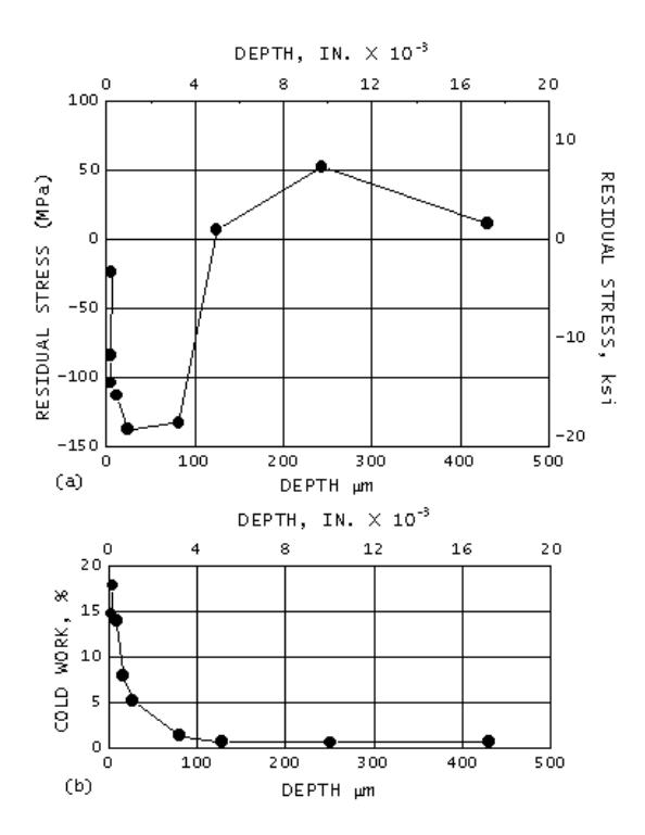
Figure 14: Longitudinal Residual Stress and Percent Cold Work Distributions in Belt-Polished Inconel 600 Tubing

The subsurface longitudinal residual stress and percent plastic strain distributions were determined by electropolishing thin layers of material in complete cylindrical shells from around the circumference of the 16- mm (0.625-in.) nominal diameter tubing. Layer removal began with 0.005-mm (0.0002-in.) thick layers near the sample surface, the increment between layers increasing with depth to nominally 0.4 mm (0.017 in.) beneath the original surface. Corrections were applied for penetration of the radiation to the stress gradient and for stress relaxation in the layers exposed by material removal.

The subsurface longitudinal residual stress and percent cold work distributions are shown in Figure 14. The residual stress distribution shows a pronounced gradient from approximately -35 MPa (-5 ksi) at the surface to a maximum compressive value of approximately -150 MPa (-20 ksi) at a nominal depth of 0.05 mm (0.002 in.). With increasing depth, the stress distribution rises back into tension at approximately 0.13 mm (0.005 in.), with a low-magnitude equilibrating tensile maximum of nominally 55 MPa (8 ksi) at greater depths. The cold work distribution shows a slight hook near the surface of the sample with a maximum of 19% at a nominal depth of 5 μm (0.0002 in.). With increasing depth, the cold-work distribution decreases nearly exponentially to negligible values beyond approximately 0.13 mm (0.005 in.) beneath the belt-polished surface.

A 63-mm (2.5-in.) U-bend manufactured from Inconel 600 tubing was strain gaged at the apex and sectioned to remove approximately a 50 mm (2 in.) arc length. This portion of the U-bend was mounted in a special fixture providing precision orientation around the circumference of the tubing to an accuracy of 0.1°. X-ray diffraction residual macrostress measurements were made on the existing surface as a function of angle θ around the circumference of the tubing.

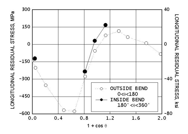
Figure 15: Longitudinal Residual Stress as A Function of the Quantity (1 + Cos Θ) For A 63-Mm (2.5-In.) Inconel 600 Tubing U-Bend

 

The longitudinal surface residual stress distribution around the bent tubing is shown in Figure 15. The stress is plotted as a function of the quantity (1 + cos θ) to expand the central portion of the plot, at which the sharp transition occurs between maximum compression and tension. The position around the circumference of the tubing ranges from the outside of the bend at the origin, around the flank to the neutral axis at (1 + cos θ) = 1, and around to the inside of the bend at 2.0. The results shown as open circles indicate the longitudinal residual stress around one side of the tubing; closed circles indicate comparable measurements made on the opposing side.

The x-ray beam was limited to a height of 0.5 mm (0.020 in.) and a width of 2.5 mm (0.1 in.) along the axis of the tubing. The small beam size was necessary to optimize spatial resolution in the presence of the pronounced stress gradient occurring on the flank of the tubing. The compressive stresses produced around the outside of the bend exceed -550 MPa (-80 ksi) in a material with a nominal annealed yield strength of 240 MPa (35 ksi). The presence of these high stresses after forming result from cold working at the tubing induced during belt polishing. Cold working of Inconel 600 to 20% increases yield strength to approximately 690 MPa (100 ksi). Cold-worked surface layers in components subjected to subsequent forming frequently result in complex residual stress distributions having magnitudes often exceeding the yield strength of the undeformed material.

Example 3: Local Variations in Residual Stress Produced by Surface Grinding. The high spatial resolution of x-ray diffraction residual stress measurement was applied to determine the longitudinal surface and subsurface residual stress variation near grinder bums produced by traverse grinding of a sample of 4340 steel with a hardness of 50 HRC. Three samples were initially investigated: two were ground abusively to produce grinder burn, and one was ground gently using adequate coolant. X-ray diffraction residual stress measurements were performed initially on only the surfaces of the three samples using a Cr Kα (211) two-angle technique. The diffraction-peak positions were located using a five-point parabolic regression procedure, assuming the Kα doublet to be completely blended into a single symmetrical peak for all measurements performed in the hardened material. The irradiated area was 0.5 by 6.4 mm (0.020 by 0.250 in), with the long axis aligned in the grinding direction. Measurements were conducted using the narrow irradiated area as a function of distance across the surface of each sample. A single measurement using a 12.5-by 6.4-mm (0.5- by 0.250-in.) irradiated area spanning nearly the entire region covered by the series of measurements made with the smaller irradiated zone was then performed on each sample.

Figure 16 shows the results of the surface measurements. The individual measurements made using the 0.5-mm (0.02- in.) wide irradiated area are shown as open circles. The single result obtained using the large13-mm (0.5-in.) wide beam is plotted as a dashed line. The bounds on the line indicate the approximate extent of the large irradiated area. The gently ground sample C was found to be uniformly in compression, with surface stresses ranging from approximately -400 to -520 MPa (-60 to -75 ksi) at all points examined. The measurement made with the large irradiated area equals the arithmetic average over the region, as expected for the combined diffracting volume.

 

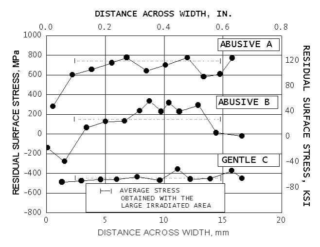
Figure 16: Variations in Longitudinal Surface Residual Stress Produced by Surface Grinding 4340 Alloy Steel (50 HRC) Samples

 

The subsurface residual stress distribution was then determined at the points of maximum compression and maximum tension on the abusively ground sample B using the 0.5-mm (0.020-in.) irradiated area. The sample was electropolished completely across the width as measurements were conducted at the two locations of interest. The subsurface results shown in Figure 17 indicate compressive stresses near the edge of the unburned sample at the point of maximum surface compression that extend to a nominal depth of 0.05 mm (0.002 in.), and then rise into tension approaching 500 MPa (70 ksi) at greater depths. The burned region shows entirely tensile stresses ranging from approximately 275 to 345 MPa (40 to 50 ksi) to a depth of 0.05 mm (0.002 in), and then rises into tension of approximately 600 MPa (90 ksi) further below the surface.

The residual stresses produced by many grinding and machining operations can vary significantly over local distances, particularly if there is significant heat input caused by loss of coolant or friction from dull tooling. As seen in Figure 17, a nondestructive surface measurement of residual stress may not reveal subsurface tensile residual stresses that could severely degrade fatigue performance.

Example 4: Longitudinal Residual Stress Distribution in Welded Railroad Rail. Continuously welded railroad rail may be subject to high tensile or compressive applied stresses resulting from seasonal thermal contraction and expansion in the field as well as cyclic loading of the rolling cars. Rail fatigue failure at the welded joints is a primary cause of derailments. Residual stresses in the flash butt welded joints of the continuously welded rail add a residual mean stress which can contribute to fatigue failures initiating near the welds. The head of modern rail is also often hardened to minimize wear, particularly for rail installed at curves where the wheel may slide on the top of the rail. To determine the longitudinal residual stresses in the hardened head of welded rail in the vicinity of the weld, a nominally 200 mm (8 in.) portion of rail containing the weld was band sawed from a section of continuous rail after butt welding. Sectioning stress relaxation was assumed to be negligible.

The residual stresses produced by many grinding and machining operations can vary significantly over local distances, particularly if there is significant heat input, loss of coolant, or tool dulling. Further, use of a nondestructive surface measurement of residual stress or a nital etch to reveal grinder burn may not reveal subsurface tensile residual stresses that could degrade fatigue performance severely

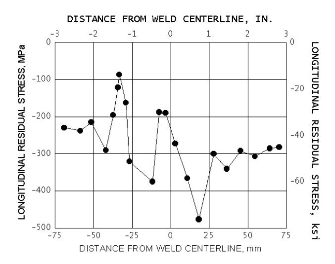
Figure 18: Longitudinal Residual Stress Distribution across a Flash Butt Welded Induction-Hardened Railroad Rail Head

 

The surface of the rail head was prepared by electropolishing to a nominal depth of 0.25 mm (0.010 in.) to remove any surface residual stresses that may have originated from sources other than welding. X-ray diffraction longitudinal residual stress measurements were then conducted using the two-angle technique at a series of positions across the center line of the weld, which was located by etching with nital before electropolishing. A Cr Kα (211) technique was used, locating the diffraction peak using a parabolic regression procedure. The rail head was induction hardened, and the Kα doublet was completely blended and symmetrical throughout the hardened head portion of the rail.

The longitudinal residual stress distribution is shown in Figure 18. The longitudinal residual stress distribution in head of the rail is entirely compressive near the weld, revealing an asymmetrical oscillating pattern of residual compression different from what would have been predicted by analytical solution for a uniformly fused and cooled simple butt joint. The results of repeat measurements confirmed the nature of the stress distribution.

The analytical methods for predicting the residual stresses produced by welding generally predict a symmetrical residual stress distribution around the weld fusion line; however, the actual stress distributions revealed by measurement are often substantially more complex than those predicted. The complexity may be due to deformation of the hot weld and heat affected zones during the cooling stages of the mechanized field welding process.

Example 5: Determination of the Magnitude and Direction of the Maximum Residual Stress Produced by Machining. The direction of maximum residual stress, that is, most tensile or least compressive, is assumed to occur in the cutting or grinding direction during most machining operations. This is frequently the case, but the maximum stress often occurs at significant angles to the cutting direction. Furthermore, the residual stress distributions produced by many cutting operations, such as turning, may be highly eccentric, producing a highly tensile maximum stress and a highly compressive minimum stress.

The residual stress field at a point, assuming a condition of plane stress, can be described by the minimum and maximum normal principal residual stresses, the maximum shear stress, and the orientation of the maximum stress relative to some reference direction. The minimum stress is always perpendicular to the maximum. The maximum and minimum normal residual stresses, shown as σ1 and σ2 in Fig. 2, and their orientation relative to a reference direction can be calculated along with the maximum shear stress using Mohr’s circle for stress if the stress σφ is determined for three different values of φ.

To investigate the minimum and maximum normal residual stresses and their orientation produced by turning an Inconel 718 cylinder, x-ray diffraction residual stress measurements were performed in the longitudinal, 45°, and circumferential directions at the surface and at subsurface layers to a nominal depth of 0.1 mm (0.004 in.), exposing the subsurface depths by electropolishing complete cylindrical shells around the cylinder. The cylinder was nominally 19 mm (0.75 in.) in diameter and uniformly turned along a length of several inches. The irradiated area was limited to a nominal height of 1 mm (0.05 in.) around the circumference by 2.5 mm (0.10 in.) along the length. Measurements were conducted using a Cu Kα (420) two-angle technique, separating the Kα1, peak from the doublet using a Pearson VII peak profile.

 

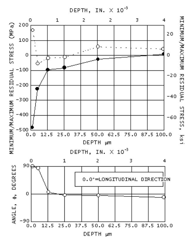Figure 19: Minimum and Maximum Principal Residual Stress Profiles and Their Orientation Relative to the Longitudinal Direction in a Turned Inconel 718 Cylinder

 

The measurements performed independently in the three directions were combined using Mohr’s circle for stress at each depth to calculate the minimum and maximum normal residual stresses and their orientation defined by the angle φ, which was taken to be a positive angle counterclockwise from the longitudinal axis of the cylinder. Figure 20 illustrates the results, showing the maximum and minimum principal residual stress profiles and their orientation relative to the longitudinal direction. The maximum stresses are tensile at the surface, in excess of 140 MPa (20 ksi), dropping rapidly into compression at a nominal depth of 0.005 mm (0.0002 in.). The maximum stress returns into tension at depths exceeding 0.025 mm (0.001 in.) and remains in slight tension to the maximum depth of 0.1 mm (0.004 in.) examined. The minimum residual stress is in compression in excess of -480 MPa (- 70 ksi) at the turned surface and diminishes rapidly in magnitude with depth to less than -138 MPa (-20 ksi) at a depth of 0.013mm (0.0005 in.). The minimum stress remains slightly compressive and crosses into tension only at the maximum depth examined. The orientation of the maximum stresses is almost exact in the circumferential direction (90° from the longitudinal) for the first two depths examined. For depths of 0.013 mm (0.0005 in.) to the maximum depth of 0.1 mm (0.004 in.), the maximum stress is within approximately 10° of the longitudinal direction.

The results appear to indicate that stresses within approximately 0.013 mm (0.0005 in.) of the sample surface are dominated by machining, which resulted in a maximum stress direction essentially parallel to the cutting action. At greater depths, the stress distribution may be governed not by the machining as much as by stresses that may have been present due to forging or heat treatment.

Example 6: Optimizing Residual Stress and Cold Work in Shot Peening. Shot peening is by far the most widely used surface enhancement process used to improve fatigue performance. Shot peening is controlled by selection of a shot material and size, and the peening intensity measured by deflection of an Almen strip to produce a required coverage. Coverage is generally at least “100%”, meaning essentially all of the surface is impacted and dimpled by shot. Often more than 100% is used in an attempt to ensure that every point on the surface is impacted.

Figure 20: Subsurface Residual Stress Distributions in 4340 Steel, 50 HRC Shot Peened at 3% To 200% Coverage

 

Excessive coverage can damage the surface, reduce ductility, increase costs, and reduce production rates without further fatigue performance benefit. The Almen strip serves the intended purpose as a measure of the peening apparatus operation, but it is manufactured from 1070 steel, and heat treated so that it neither work hardens or softens. It does not reveal the actual residual stress or cold work developed in the shot peened component. Subsurface XRD residual stress and cold work measurements made on the shot peened component can be used to determine the minimum coverage needed to achieve the depth and magnitude possible for a given peening process.

The subsurface residual stress and cold work distributions produced in 4340 steel, 50 HRC, by shot peening with 3% to 200% coverage with cut wire 14 shot at 9A intensity are shown in Figure 20. The large number of measurements shown were obtained with an automated electropolishing apparatus developed at Lambda Research mounted on an automated diffractometer. The full depth and magnitude of the beneficial compressive layer is achieved with minimal cold work with as little as 20% coverage. The regions between the peening dimples are in compression, as has been confirmed by finite element modeling and fatigue testing. Further coverage only produces more cold work, but gives no further residual compression or fatigue benefit. Because of the random nature of shot impacts full coverage is approached exponentially, with 80% coverage achieved in only 20% of the peening time. Therefore, production rates can be increased 5-fold by peening to 80% rather than 100% coverage. Optimizing peening processes using XRD stress and cold work measurements can improve production rates and reduce costs without sacrificing fatigue performance.

Example 7: Prediction of Yield Strength Gradient and Residual Stress Inversion from Plastic Deformation Fatigue critical areas of components subject to low cycle fatigue (LCF), such as compressor and turbine disks, are frequently shot peened to introduce a layer of compression to improve fatigue performance. Disk bores and dovetail slots will yield, usually a fraction of a percent, with each cycle at the high LCF service loads. If the yield strength of the surface material has been altered by cold working during shot peening, benefit of the compressive layer from shot peening may be lost, or even inverted into tension when the softer, less compressive subsurface material yields.

The surface layers of a metallic component are plastically deformed and cold worked by machining, grinding, shot peening, or other mechanical processing. As noted above, the dislocation density and lattice strain range increase from cold working. In a work hardening alloy, the yield strength increases in relation to the degree of cold working induced at each depth. The amount of cold work can be measured as a function of depth during electropolishing for subsurface XRD residual stress measurement. Defining the measure of “cold work” as the equivalent amount of true plastic strain required to produce the line broadening measured, a true stress-strain curve extending to the plastic strain levels produced by the processing can be used to determine the change in yield strength at each depth.

The effect of 2% tensile plastic deformation on the beneficial compressive layer produced by shot peening of a nickel base disk super alloy tensile sample was measured and compared to the original compressive profile before deformation. The yield strength at each depth was estimated from the available true stress-strain curve. Finite element analysis was then used with the yield strength gradient applied at each depth to predict the change in the residual stress distribution due to 2% plastic deformation.

 

Figure 21: Subsurface Residual Stress, Cold Work and Yield Strength Distributions Show Inversion to Tension With 2% Extension and FEA Confirmation

 

The residual stress distributions as-shot peened and after 2% plastic elongation are shown in Figure 21. The highly compressive spot peened layer was inverted from over -1000 MPa to tension approaching +400 MPa in a single half-cycle, comparable to an LCF limited turbine engine reaching full RPM for the first time. The cold work measured by XRD line broadening and the yield strength gradient estimated from the true stress-strain curve are as functions of depth in the bottom of Figure 21. The FEA prediction with the yield strength gradient was in remarkably good agreement with the measured residual stress after 2% elongation. The variation in yield strength was found to dominate the FEA prediction, and the existing compressive residual stress distribution had little influence.

Example 8: Mapping Residual Stresses Distributions from Welding Welding can develop complex residual stress distributions that may include local areas of high residual tension that leave the welded assembly subject to fatigue or stress corrosion failure. The residual stresses developed upon cooling are determined by the temperature distribution and properties of the weld metal, heat affected zones and parent metal as functions of time, and the physical constraints imposed on the structure. The order of welding determines both the temperature distributions over time and the constraints as different portions of the weld fuse and contract upon cooling. The combination of variables can be very difficult to predict. XRD residual stress measurements made using automated sample or instrument positioning can be programmed to perform a series of measurements in a grid pattern. Contour maps of the complex stress distributions can then be created.

 

Figure 22: Contour Map of the Residual Stress Distribution Produced In a T-Weld of Three Steel Plates

 

A contour map of the residual stress parallel to the x-axis of a “T” weld is shown in Figure 22. The weldment was made from the three pieces of plate shown. Welds were made in the directions shown, with the first weld attaching the two 30x40mm plates to the upper plate, welding from left to right. The final 30 mm vertical weld joined the two smaller plates.

Residual stress measurements were made in the direction parallel to the X-axis using an automated X-Y positioning stage programed to perform measurements at 5mm increments. Measurements were not made in the fusion zone of the weld because of the coarse grain size and irregular surface topography. The contour plot reveals that the highest stress occurs on either side of the final vertical weld in both of the smaller plates. However, the maximum stress, over 500 MPa occurs to the left of the final weld in the first small plate that was constrained by the initial horizontal weld. The small plate and the portion of the weld on the left had more time to cool before the final vertical weld was made. Yield strength of the material would then be higher as the final weld cooled and contracted, allowing higher residual stresses to be developed on the left side of the weld. The upper plate is seen to be drawn into equilibrating compression by the tensile zone across the lower vertical weld.

General References

1. A. Ahmad, P. Prevéy, and C. Ruud, Ed., SAE Residual Stress Measurement by X-Ray Diffraction, SAE HS-784, SAE International, Warrendale, PA, 2003.

2. I.C. Noyan and J.B. Cohen, Residual Stress Measurement by Diffraction and Interpretation, Springer-Verlag, NY, 1987

3. European Committee for Standardization (CEN), BS EN 15305:20008, Non-Destructive Testing—Test Method for Residual Stress Analysis by X-ray Diffraction, British Standards Institute, 2009

4. J. Lu, Ed., Handbook of Measurement of Residual Stresses, Fairmont Pr, 1996

REFERENCES

1. M.E. Hilley, Ed., Residual Stress Measurement by X-Ray Diffraction, SAE J784a, Society of Automotive Engineers, Warrendale, PA, 1971, p 21-24
2. B.D. Cullity, Elements of X-Ray Diffraction, Addison Wesley, 2nd ed., 1978, p 470
3. M.E. Hilley, Ed., Residual Stress Measurement by X-Ray Diffraction, SAE J784a, Society of Automotive Engineers, Warrendale, PA, 1971, p 19
4. M.E. Hilley, Ed., Residual Stress Measurement by X-Ray Diffraction, SAE J784a, Society of Automotive Engineers, Warrendale, PA, 1971, p 20
5. R.H. Marion and J.B. Cohen, Adv. X-Ray Anal., Vol 18, 1975, p 466
6. P.S. Prevéy, Adv. X-Ray Anal Vol 19, 1976, p 709
7. H. Dölle and J.B. Cohen, Met. Trans., Vol 11A, 1980, p 159
8. H. Dölle, J. Appl. Cryst., Vol 12, 1979, p 498
9. M.E. Hilley, Ed., Residual Stress Measurement by X-Ray Diffraction, SAE J784a, Society of Automotive Engineers, Warrendale, PA, 1971, p 61
10. A.L. Christenson and E.S. Rowland, Trans. ASM, Vol 45, 1953, p 638
11. D.P. Koistinen and R.E. Marburger, Trans. ASM, Vol 51, 1959, p 537
12. W.A. Rachinger, J. Sci. Instr., Vol 25, 1948, p 254
13. S.K. Gupta and B.D. Cullity, Adv. X-Ray Anal., Vol 23, 1980, p 333
14. P.S. Prevéy, Adv. X-Ray Anal., Vol 29, to be published
15. “Standard Method for Verifying the Alignment of Xray Diffraction Instrumentation for Residual Stress Measurement,” E 915, Annual Book of ASTM Standards, Vol 03.01, ASTM, Philadelphia, 1984, p 809-812
16. “Standard Methods for Determining Average Grain Size,” E 112, Annual Book of ASTM Standards, Vol 02.01, ASTM, Philadelphia, 1984, p 1073-1107
17. P.S. Prevéy, Adv. X-Ray Anal., Vol 20, 1977, p 345
18. M.G. Moore and W.P. Evans, Trans. SAE, Vol 66, 1958, p 340

 

Table 1 Recommended diffraction techniques, x-ray elastic constants, and bulk values for various ferrous and nonferrous alloys

(a) Constants determined from four-point bending tests.

(b) K45 is the magnitude of the stress necessary to cause an apparent shift in diffraction-peak position of 1° for a 45° angle tilt